SOQCS Example 9: Dielectric film with losses.

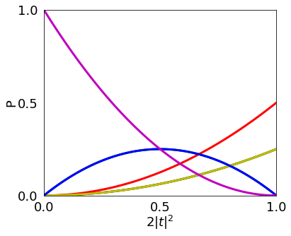
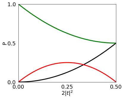
We consider a circuit made of single dielectric thin film as studied in [1]. We reproduce numerically the results presented in figs 2 and 3 of the same ref. [1] obtained by means of analytical calculations to validate the loss model in SOQCS. Each of the figures correspond to the cases where two photons are injected in the dielectric from the same direction or from opposite directions. Here, both situations are considered as two different input channels therefore we plot the different outcome probabilities as function of the transmission amplitude |t| for each of the two cases | 2, 0 > and | 1, 1 >.

[1] Stephen M. Barnett, et Al. Quantum optics of lossy beam splitters. Physical Review A Volume 57 Number 3 (1998)

[1]:

import soqcs         # Import SOQCS
import numpy as np   # Import numpy

Build the plotting function for a | 2, 0 > input.

SOQCS Circuit.

Next, we build a function that contains the calculation of the output probability of the dielectric given a transmission amplitude t for the case when the input is \(|2, 0 >\). The probability is calculated for a specific outcome. Its occupation is provided to the function as parameters. Note: This is not the most efficient implementation. All the objects have to be recreated for each point calculation and only one probability is returned at a time (even if various have been calculated). This code is implemented for demonstration purposes therefore it is intended to be simple.

[2]:

def DieProb(x,args):
    #Obtain t
    t=np.sqrt(x/2.0)
    #Build the circuit
    example = soqcs.qodev(nph=2, nch=2, nm=1, ns=2, clock=0, R=0, loss=True)
    example.add_photons(2,0,0, 0.0, 1.0,1.0)
    example.dielectric(0,1,t,1j* t)
    example.detector(0);
    example.detector(1);

    # Create a simulator and run the simulation
    sim=soqcs.simulator()
    measured=sim.run(example)

    term=[[0      ,      1],
          [args[0],args[1]]]
    prob=measured.prob(term,example)
    return prob

Results.

\(| 2, 0 >\): Black
\(| 1, 1 >\): Red
\(| 1, 0 >\): Green
\(| 0, 2 >\): Yellow
\(| 0, 1 >\): Blue
\(| 0, 0 >\): Purple

Some colors may not be vissible if two plots are the same ( for example | 2, 0 > and | 0, 2 > ).

[3]:

      #Arg1  #Arg2
args=[{0:2,  1:0},  #Plot 1
      {0:1,  1:1},  #Plot 2
      {0:1,  1:0},  #Plot 3
      {0:0,  1:2},  #Plot 4
      {0:0,  1:1},  #Plot 5
      {0:0,  1:0}]  #Plot 6

soqcs.plot(DieProb,6,5,'$2|t|^2$', 0.0, 0.9999, 3 ,'P', 0.0 , 1.0, 3, 100, args,['k','r','g','y','b','m'])

Build the plotting function for a | 1, 1 > input.

Individual function

Next, we build a function that contains the calculation of the output probability of the dielectric given a transmission amplitude t for the case when the input is \(|1, 1 >\). The probability is calculated for a specific outcome. Its occupation is provided to the function as parameters. Note: This is not the most efficient implementation. All the objects have to be recreated for each point calculation and only one probability is returned at a time (even if various have been calculated). This code is implemented for demonstration purposes therefore it is intended to be simple.

[4]:

def DieProb(x,occ1,occ2):
    # Obtain t
    t=np.sqrt(x/2.0)

    #Build the circuit
    example = soqcs.qodev(nph=2, nch=2, nm=1, ns=2, clock=0, R=0, loss=True)
    example.add_photons(1,0,0, 0.0, 1.0,1.0)
    example.add_photons(1,1,0, 0.0, 1.0,1.0)
    example.dielectric(0,1,t,t)
    example.detector(0,);
    example.detector(1);

    # Create a simulator and run the simulation
    sim=soqcs.simulator()
    measured=sim.run(example)

    term=[[0,1],
          [occ1,occ2]]
    prob=measured.prob(term,example)
    return prob

Sum function

In this case the interest is to give the total probability of detecting at the output 0, 1 or 2 photons independently of the channel where those are detected. Therefore we need to sum the probabilities of the different outcomes that contain 0, 1 or 2 photons in each case.

[5]:

def DieSumProb(x,args):
    if(args[0]==2):
        probs1=DieProb(x,2,0)
        probs2=DieProb(x,1,1)
        probs3=DieProb(x,0,2)
        probs=probs1+probs2+probs3

    if(args[0]==1):
        probs1=DieProb(x,1,0)
        probs2=DieProb(x,0,1)
        probs=probs1+probs2

    if(args[0]==0):
        probs=DieProb(x,0,0)

    return probs

Plotting the function

\(| 2 >\): Black
\(| 1 >\): Red
\(| 0 >\): Green

[6]:

soqcs.plot(DieSumProb,6,5,'$2|t|^2$', 0.0, 0.5, 3 ,'P', 0.0 , 1.0, 3, 100, [{0:2},{0:1},{0:0}],['k','r','g'])

THIS CODE IS PART OF SOQCS

Copyright: Copyright © 2023 National University of Ireland Maynooth, Maynooth University. All rights reserved. The contents and use of this document and the related code are subject to the licence terms detailed in LICENCE.txt